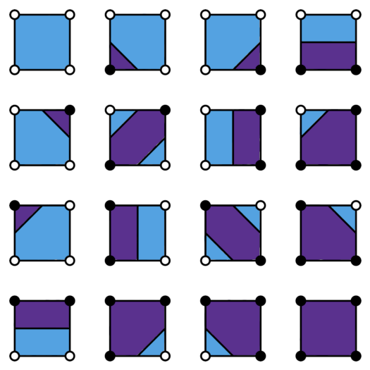
The 16 possibilities for rendering cells, with blue for empty space and
purple for filled areas
Git repository: Link
Yusuke Endoh's original:
IOCCC
Invidious Youtube
One of the submissions for the 2012 International Obfuscated C Code Contest was a 23, 30, or 31 line piece of seeming nonsense code that did... something. When fed appropriately sized text as input, all characters except for instances of '#' would melt and flow as if liquid. It was a fluid simulator that worked with ASCII text in the terminal.
While it didn't win, it did receive an honorable mention and has also attracted the occasional article over the years since then. Often with commenters in awe of how it does what it does. Because it is damned cool.
So it's doing some sort of black magic to accomplish this, right? Well, yes, but also no. Condensing and obfuscating the code to fit in 23 lines as in the original monochrome version is definitely some impressive magic. But actually simulating a fluid in textual form is surprisingly easy. What's going on is it's running a simplified version of smoothed-particle hydrodynamics which involves nothing more complicated than addition, subtraction, multiplication, division, exponentiation, and square roots. And technically also complex numbers, because they tend to be the most accessible way to deal with two dimensional values. Nothing too difficult.
To prove how easy it is, the rest of this article is going to detail what you need to know so that you too can write your very own comprehensible knockoff version.
First thing to note is what we are dealing with. Every particle is stored as a structure containing five values:
These particles can be stored in whatever convenient data structure you like. The most natural is probably a vector since the program isn't sure how much input it is going to be given, but an array can also be made to work.
Reading in the input is just done with standard text I/O functions. But here is a very important detail to note: Each character of ASCII input actually denotes two particles, one just above the other in position. That is, while the input is usually a textfile with no more than 25 rows, once it is read into the program you will have double the number of particles spread across an 80x50 field. The display algorithm will scale it back to 25 later on.
If you do not double up the input like this, your simulator will still work, but it won't look quite right. Details like how high particles bounce will be off.
Also note that by typical terminal conventions, coordinates (1,1) are at the top left corner and numbers increase as you go down and right. Following this convention will make reading in input easier, but will have some implications for gravity.
Before going into the physics calculations, there are a handful of useful constants that are going to be needed:
Note that while the gravitational constant magnitude is set to 1, care still has to be taken to make sure the value is oriented in the correct direction. If terminal conventions are being followed for axis orientation then the value will actually be the complex number . Endoh avoids this issue by switching the axes.
Also note that while the documentation for Endoh's simulator claims the gravitational, pressure, and viscosity parameters are set to 1, 4, 8 as they are here, there is actually an error in his makefile. As a result the viscosity constant is set equal to the pressure constant, causing them to take on values of 1, 4, 4 by default instead.
The density of each particle can be calculated by:
Or in other words, for each particle, find all the other particles within a radius of 2, weight the distance between the two by the function, multiply by the particle mass of 1, and sum up all these intermediate results. That's the particle's density.
Particles that are part of a solid wall get an additional density of 9, so don't forget to add that too.
It is recommended that you do this step before you render any output results since you may want to use density values to color the output. Endoh's simulator doesn't bother, however.
The acceleration of each non-wall particle is the sum of two components, gravity and interaction forces. Gravity is very simple as it is just the gravitational constant already defined earlier. The interaction forces acting on each particle can be calculated by:
A lot to take in, I know. A bit too much to rephrase in plain english this time, even though it is a simplified form compared to the usual smoothed-particle hydrodynamics formula. But as promised, once you get past all the variables there is still only elementary math involved.
So, the gravity plus the interaction force. That's the particle's acceleration.
Acceleration of non-wall particles can be ignored since they will never move and the value won't have any affect on other calculations.
As implemented in Endoh's simulator this is by far the easiest step. For each non-wall particle, merely divide the acceleration value by 10 then add that to the velocity value. Then add the velocity to the particle's position. The division by 10 is an arbitrary scaling factor to make things work in the space a standard 80x25 size terminal gives us.
If you want to go the extra mile and add collision detection between moving particles and wall particles, this would be the step to implement it. I haven't bothered. Partially because collision detection is tricky, but also because doing so would result in visibly different behaviour.
Believe it or not, this is actually the most complicated part of this whole thing. It might be fairly easy to explain in concept, but the actual implementation is more finnicky than any of the previous steps.
The algorithm in use here is called Marching Squares. You calculate whether there are any particles present at the corners of each character cell on an 80x25 terminal, then use those results to look up which character should go in that cell from a predetermined mapping of cases to output characters. Some experimentation may be required to find characters that look close enough, as the ASCII character set was not made with this in mind.
Be sure to scale the vertical axis back down by a factor of 2 before you perform these calculations in order to take the input doubling into account.
Various small tricks with bitwise-or operations can be used to make this process more efficient, but going into those is beyond the scope of this article.
To clear the screen and reset the cursor between output renders, ANSI escape codes are used. They are also used if you want to add color to the output, with an escape code inserted before each character to change the color according to the average density of the particles contributing to that cell. Since the escape codes to do this are quite long, the resulting string will get decently large. It won't affect the size when displayed to the terminal, however.
In my experience, the average density in a given cell usually remains in the range 0-20 unless in the middle of a thick solid wall. Scaling the colors used to that range tends to work well.
The entire program consists of reading in the input, then looping through calculating density, rendering output, calculating acceleration, and updating the particle positions. That's really it. The only other thing you will probably want to do is have some step to get rid of particles should their position go too far off-screen. Both to avoid unnecessary computation and the potential for values to overflow and cause an error.
The calculation and update steps are all embarrassingly parallel, so if you're looking for places to improve things beyond adding color then there would be a good place to start. Neither Endoh's implementation nor mine do anything with that, but that is more due to lack of need to put in the effort.
Now, was this entire exercise ultimately pointless, since it is concerned with ASCII rendering done by intentionally obfuscated code? Yes. Was it nonetheless interesting and fun? Also yes.
Thank you Daniele Venier for your informative, if incomplete, article on this same topic which let me avoid having to analyse the IOCCC entry from scratch myself. Although really, it probably would have still been easier to construct something from first principles anyway.
{% endblock -%}