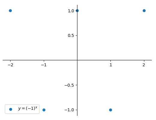
Figure 1 - Real values only
Scripts used to generate graphs: Link
A definite integral can be represented on the xy-plane as the signed area bounded by the curve of the function f(x), the x-axis, and the limits of integration a and b. But it's not immediately clear how this definition applies for complex valued functions.
Consider the following example:
If the function is graphed on the xy-plane, the real valued outputs are sparse. Yet an elementary antiderivative exists and the definite integral is well defined.
In order to plot a meaningful graph that can be used to potentially calculate the integral as a signed area, some cues are taken from Philip Lloyd's work on Phantom Graphs. In that work, an additional z-axis is used to extend the x-axis into a complex xz-plane, allowing complex inputs to be graphed. For the function considered here, the z-axis is instead used to extend the y-axis into a complex yz-plane to allow graphing of complex outputs instead.
Upon doing so, the following helical graph is obtained:
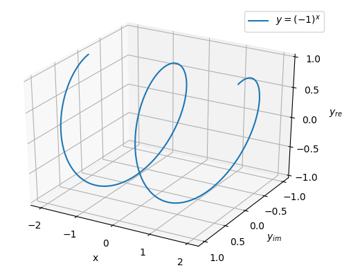
The curve is continuous and spirals around the x-axis, intersecting with the real xy-plane at the points plotted in the initial graph of Figure 1. However it is still not clear how to represent the area under the curve.
Observing that complex numbers in cartesian form are composed of a real part and an imaginary part, it is possible to decompose the function into real and imaginary components. These are easy to obtain by rotating the graph above to view the real and imaginary parts as flat planes.
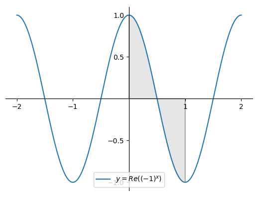
Figure 3 - Real component
|
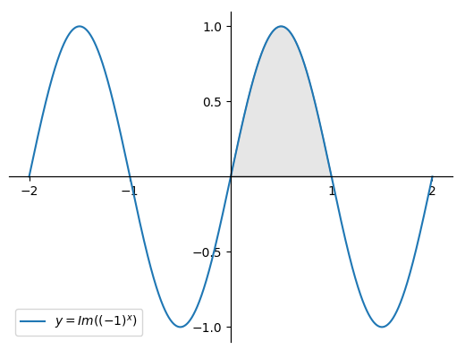
Figure 4 - Imaginary component
|
From this it can be seen that the function is a combination of a real valued cosine and an imaginary valued sine. With the limits of integration under consideration, the real values disappear and we are left with the following:
| = | |
| = | |
| = | |
| = | |
This agrees with the answer obtained by ordinary evaluation of the integral without considering the graph, so the informal area under the curve definition still works. Considering the area under the curve using polar coordinates also works, but requires evaluating a less than pleasant infinite sum and so won't be considered here.
The next interesting question is how this relates to the surface area of a right helicoid.
{% endblock -%}